library(tidyverse)
library(HDSinRdata)
library(kableExtra)
library(gt)

data(NHANESsample)22 Writing Reports in Quarto
This chapter introduces you to Quarto, which is a document format that combines Markdown text with code. Writing in Quarto helps you write reproducible code and create polished reports to present your analyses. Quarto is similar to R Markdown but is compatible with other programming languages and incorporates some new features that make it easier to write nice reports. If you already use R Markdown, it’s easy to transition to Quarto.
22.1 Starting a Quarto File
To create a Quarto file, you need to have RStudio installed as an application. For more recent versions of RStudio, Quarto is already installed. If you have an older version, you can install Quarto. We also recommend the kableExtra package (Zhu 2021) for formatting your tables.
Now that you have these packages downloaded, opening a new Quarto file is very similar to opening a new R file, which was covered in Chapter 1. Just like opening a new R file, you’ll want to go to File -> New File, but instead of selecting ‘R Script’, you’ll now select ‘Quarto Document…’. This should bring up a window that looks like Figure 22.1.
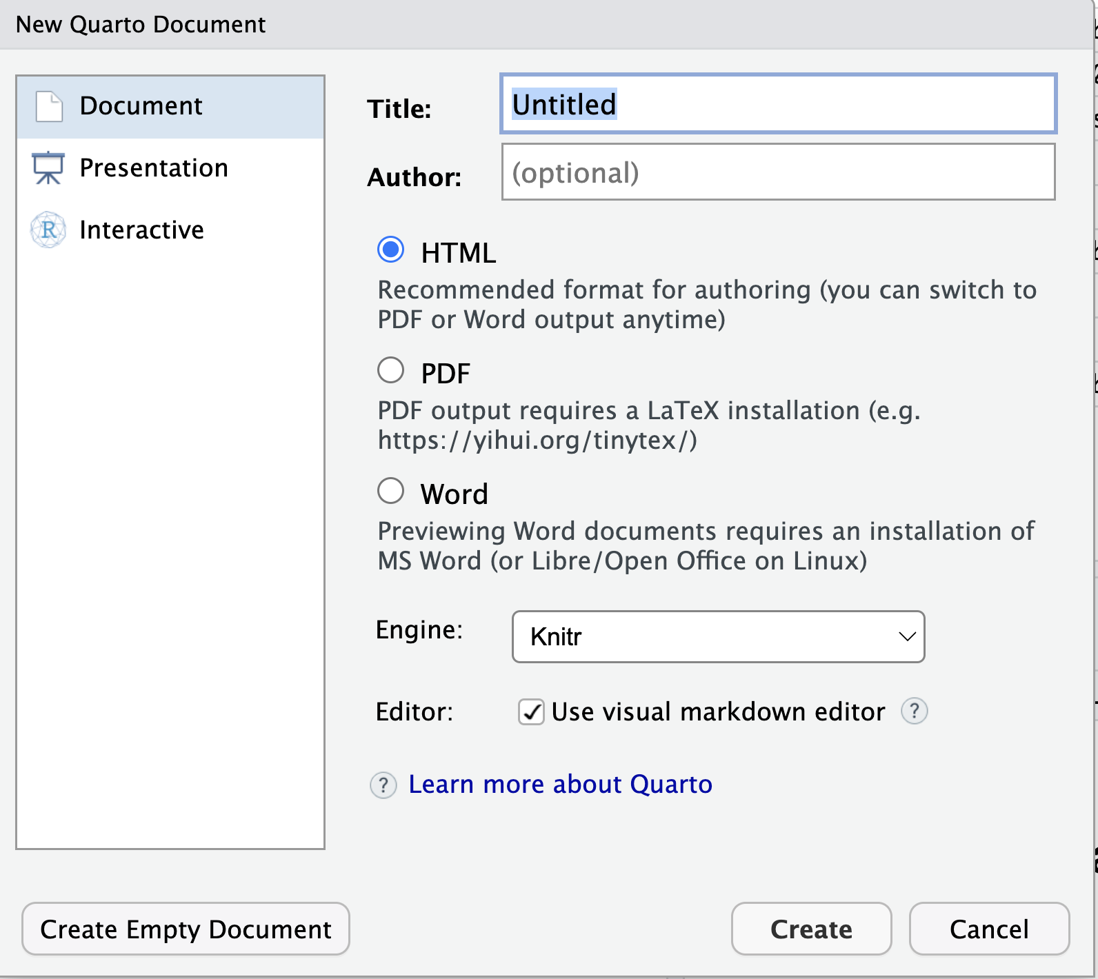
First, enter a title of your choosing for your report and type your name in the Author field (note that you can always change these later) and then click on OK. You should also choose which type of file you would like to generate, a PDF, HTML, or WORD document. This opens an Quarto file that has the extension .qmd. Make sure to save this file with a suitable name in your desired location on your computer by selecting File -> Save, and then you’re ready to start writing your report! Your file should now look like Figure 22.2.
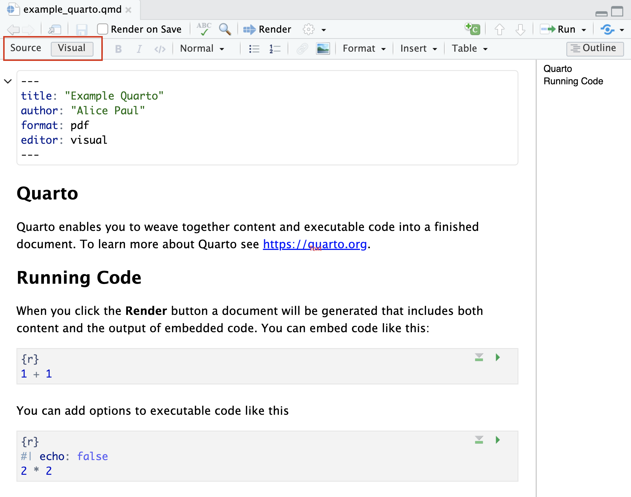
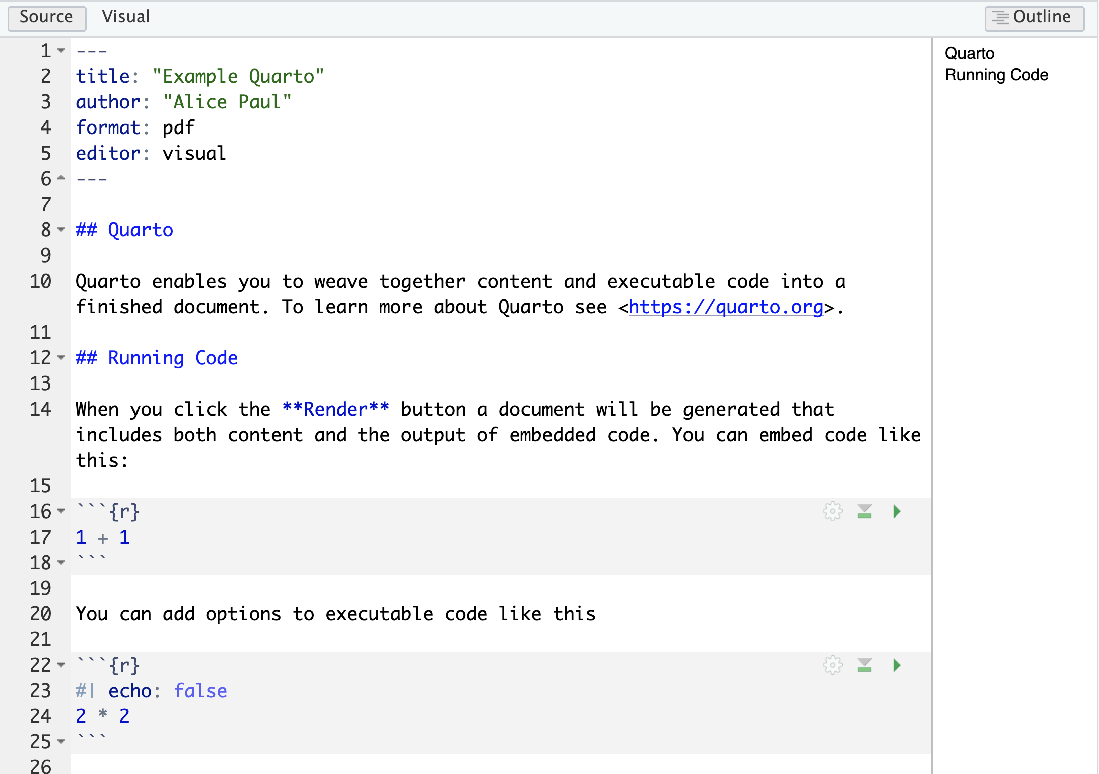
At the top of this pane is a toggle between source and visual mode. In visual mode, we can see that we have a text toolbar including options to bold text or add a list. If we switch to source mode, our text reveals the underlying Markdown in Figure 22.3 and the toolbar disappears. This chapter focuses on teaching you to edit in source mode, but you can always switch to visual mode if you prefer.
We write all of the text and code that we would like to include in your report in this .qmd file, and then produce a nicely formatted report from this file by ‘rendering’ the file. We can either render to HTML, PDF, or WORD by clicking on the Render button ![]() from the toolbar at the top of the page. To update our format from PDF, we change the text in the top block to
from the toolbar at the top of the page. To update our format from PDF, we change the text in the top block to format: html or format: word.
22.1.1 Adding Code Chunks
Each of the darker gray rectangles is called a code chunk. All of the code used to generate your report goes in these chunks, and all of your text writing goes outside of them. Each code chunk starts with ```{r} and ends with ```. To create a chunk, you can
click on this green “add chunk” symbol
 in the toolbar at the top of the page,
type
```{r}and```, oruse the keyboard shortcut Ctrl + Alt + I (Cmd + Option + I on Macs).
To run the code in a chunk, you can either use the keyboard shortcut Ctrl + Enter (Cmd + Return on Mac), or you can use one of the following buttons at the top right of the chunks:  runs all chunks above the current chunk, and
  runs the current chunk.
22.1.2 Customizing Chunks
You can specify whether you want to include the code and/or its various output in your final report by adding the following commands, preceded by #|, at the top of the code chunk:
include: falsemakes it so that neither code nor its output appears in your report.echo: falsemakes it so that the output of the code but not the code itself appears in your report.message: false,warning: false, anderror: falsemake it so that messages, warnings, and errors (respectively) that are generated from the code in the chunk won’t appear in your report.
Here we can also specify a label for our code chunk. For example, if we wanted to include a chunk that displayed our code but did not execute it, we could include the following.
  ```{r}
#| label: example-chunk
#| echo: true
#| eval: false

x <- c(1,2,3)
```
To apply the same options to all chunks in the document at once, you can add them to the first chunk at the very top of your Quarto that has the label label: setup using the knitr::opts_chunk$set() function. These are called the global settings. For example, using the following code for your first code chunk ensures that none of the errors, warnings, or messages from any of the code chunks appear in your final report. It is also good practice to load all the packages you are using for your report within this first code chunk using the library() function. For example, we load the tidyverse and HDSinRdata packages.
  ```{r}
#| label: setup
#| include: false
knitr::opts_chunk$set(warning = FALSE, error = FALSE, echo = FALSE)
library(tidyverse)
library(HDSinRdata)
```
If you want to display the code for your report in a code appendix, you can easily do this by creating an empty code chunk at the end of your .qmd file that looks like the following. This finds all other chunks and displays the code.
  ```{r ref.label = knitr::all_labels()}
#| echo: true
#| eval: false
```
22.2 Formatting Text in Markdown
To add text to your report, you can simply type directly into the Quarto file, between the code chunks. This code is formatted using Markdown, which allows us to specify how to format and display the text when it is knit. For example, adding a single asterisk * on either side of some text italicizes it, while adding a double asterisk ** on either side of text makes it bold. To indicate code, you can use backticks `.
regular text regular text
*italicized text* italicized text
**bold text** bold text
`code text` code text
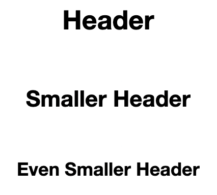
To create headers and sections, you can add the # symbol in front of your text. Adding more of these symbols makes the headers smaller, which is useful for making sub-headers (see Figure 22.4).
# Header
## Smaller Header
### Even Smaller Header
You can also add links [text](www.example.com) and images . In the latter example, fig-label becomes the label of the image we can use to cross-reference it, while image.png is the image file name (see Figure 22.5).

The Markdown Guide has a great cheat sheet as well as more resources for formatting Markdown text.
You can also have inline R code by using single backticks around your code `{r} max(c(1,2,3))`. The code must start with r to be run when knit. This allows you to reference variables in your text. For example, we could display the variance of a column in our data without having to copy the value over `{r} round(var(cars$speed),2)`.
22.3 Formatting Figures and Tables
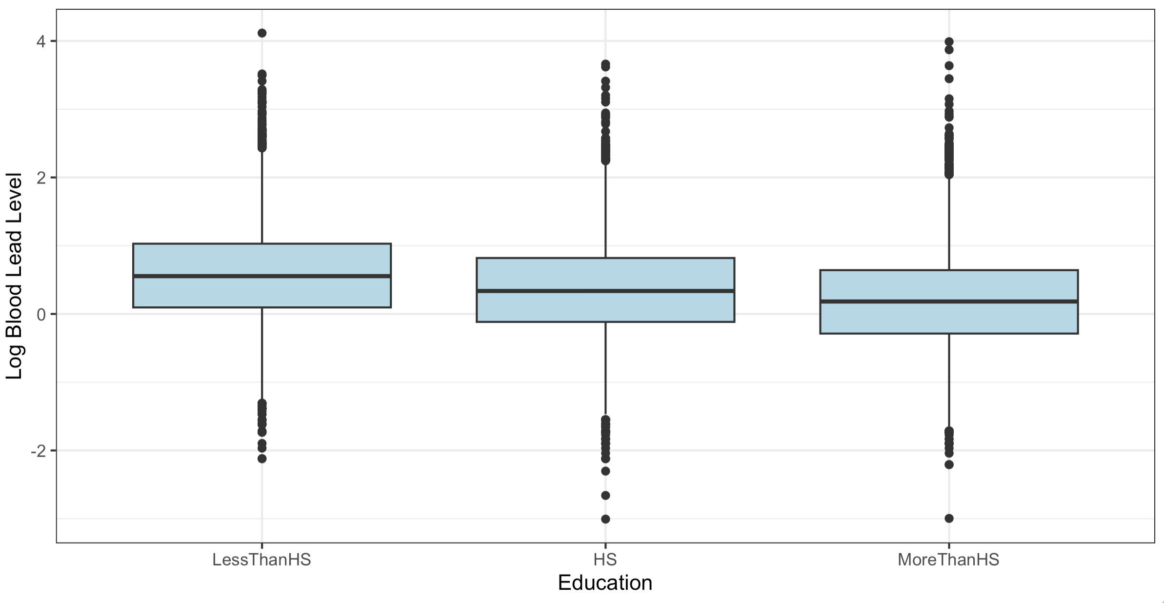
Often, you’ll want to include figures generated by your code in your report, and you can customize these figures by changing the chunk options for the chunks that produce them. To change the size of a figure, you can add in the chunk option fig-width: 3 with your desired size in inches. To add a nice caption to a figure in your report, you can add fig-cap : 'Your Desired Caption.' option. To name a figure, you want to start your label with fig- such as fig-myfigure.
By default, the figures generated by your code chunks are allowed to ‘float’ in Quarto. This means that the figures might move away from where they were coded or referenced in the final report. To prevent this behavior, you can customize the chunk that contains the code to produce the figure by adding fig-pos : 'H' to that chunk’s options. If you want to prevent floating for all figures, add fig-pos : 'H' to the first code chunk in the file (the one that starts with the knitr::opts_chunk$set() function). Figure 22.6 shows the resulting figure.
  ```{r}
  #| label: fig-myfigure
  #| fig-width: 3
  #| fig-pos: "H"
  #| fig-cap: "Blood Lead Level by Education"

  data(NHANESsample)
  ggplot(subset(NHANESsample, !is.na(EDUCATION))) +
  geom_boxplot(aes(x = EDUCATION, y = log(LEAD)), fill = 'lightblue') +
  theme_bw() +
  labs(y = "Log Blood Lead Level") +
  scale_x_discrete("Education")
  ```
If you want to make data frames, matrices, or tables from your raw R output more polished and aesthetically pleasing, you can use the gt and kableExtra packages. Be sure to load the package you are using to the code chunk at the top of your Quarto file that contains all of your libraries.
To demonstrate the abilities of these packages, let’s suppose that we wanted to display the head of the first few columns of the NHANESsample data from the HDSinRdata package. The following code produces the corresponding output in the knitted pdf report. You can see in Table 22.1 that it essentially just copies the raw output from R, which is rather messy.
NHANESsample %>%
  select(AGE, SEX, EDUCATION, INCOME, LEAD) %>%
  head()
#>   AGE    SEX  EDUCATION INCOME LEAD
#> 1  77   Male MoreThanHS   5.00  5.0
#> 2  49   Male MoreThanHS   5.00  1.6
#> 3  37   Male MoreThanHS   4.93  2.4
#> 4  70   Male LessThanHS   1.07  1.6
#> 5  81   Male LessThanHS   2.67  5.5
#> 6  38 Female MoreThanHS   4.52  1.5
We use the kable() and kable_styling() functions from the kableExtra package to produce a more nicely formatted table. The kable() function generates a table from a data frame. The kable() function allows you to specify some display options for your table. For example, you can add a caption to your table using the caption argument, and you can change the names of the columns in the table using the col.names argument. The kable_styling() has additional options available. Similar to the fig-pos = H command described for figures in the previous section, adding “HOLD_position” to the kable_styling() function prevents the table from floating on the report; adding "scale_down" scales the table so that it fits in the margins of the paper. The updated code and output are shown in the following code chunk and Table 22.2. See the documentation for the kable() and kable_styling() functions for more options available.
NHANESsample %>%
  select(AGE, SEX, EDUCATION, INCOME, LEAD) %>%
  head() %>%
  kable(col.names = c("Age", "Sex", "Education Level",
                      "Poverty Income Ratio", "Lead Level")) %>%
kable_styling(latex_options = c("scale_down", "HOLD_position"))| Age | Sex | Education Level | Poverty Income Ratio | Lead Level |
|---|---|---|---|---|
| 77 | Male | MoreThanHS | 5.00 | 5.0 |
| 49 | Male | MoreThanHS | 5.00 | 1.6 |
| 37 | Male | MoreThanHS | 4.93 | 2.4 |
| 70 | Male | LessThanHS | 1.07 | 1.6 |
| 81 | Male | LessThanHS | 2.67 | 5.5 |
| 38 | Female | MoreThanHS | 4.52 | 1.5 |
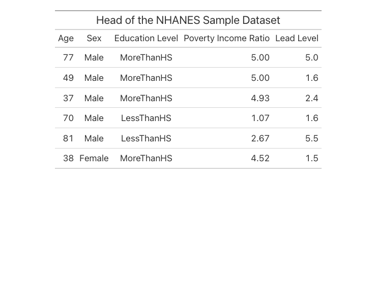
In the previous code chunk, we saw that kable() produces a much nicer table in the knitted pdf that is more suitable for a data analysis report. In Chapter 4, we also introduced the gt package. This package is an alternative package to kableExtra that allows you to format each part of the table and includes options for formatting the columns, adding footers or subtitles, or grouping your table. See the package introduction for more details about this package. An example gt table is given in the following code and output. Note that for tables, we want to start our label with tbl- and can include a caption using the tbl-cap option. The resulting table from the code chunk below is shown in Figure 22.7.
  ```{r}
  #| label: tbl-gt-ex
  #| tbl-cap: "Head of the NHANES Sample Data"

  NHANESsample %>%
  select(AGE, SEX, EDUCATION, INCOME, LEAD) %>%
  head() %>%
  gt() %>%
  tab_header(title = "Head of the NHANES Sample Data") %>%
  cols_label(AGE ~ "Age",
      SEX ~ "Sex",
      EDUCATION ~ "Education Level",
      INCOME ~ "Poverty Income Ratio",
      LEAD ~ "Lead Level")
  ```
22.3.1 Using References
Quarto automatically adds figure and table numbers to the figures and tables in your report. By using the label options, we can also reference our figures easily by using their names: @fig-figname or @tab-tablename. The knitted pdf substitutes the appropriate figure or table number into your text. Additionally, we can reference sections by adding in labels to the section header. For example, we added the tag #sec-awesome for the section in the following text and can now reference it using @sec-awesome.
## Awesome Stuff {#sec-awesome}
22.4 Adding in Equations
Another useful option in Markdown is to add in mathematical equations. If you want to insert math equations, you can do so by writing LaTeX expressions. To write a math equation inline, you put a single dollar sign $ on either side of your equation, and to write a math equation on its own line, you put a double dollar sign $$ on either side of the equation, like so:
Here’s an equation that is inline with the text: $5x^2 + 9x^3$ produces \(5x^2 + 9x^3\). On the other hand, here’s an equation that is on its own line: $$5x^2 + 9x^3$$ produces \[5x^2 + 9x^3\]
Here is some other LaTeX notation that you should know in order to write common equations: * To create a fraction, type \frac{numerator}{denominator}. For example, \frac{2}{3} produces \(\frac{2}{3}\). * To create a subscript, type _. For example, x_{2} produces \(x_2\). * To create a superscript, type ^. For example, x^{2} produces \(x^2\).
If you want to learn more about how to write in LaTeX, Art of Problem Solving provides a great reference for LaTeX symbols, and Overleaf provides a helpful introduction to LaTeX in general.
22.5 Exercises
The exercise for this chapter is to recreate this example pdf created from an Quarto file. You will need to use the NHANESsample data from the HDSinRdata package.