library(tidyverse)
library(HDSinRdata)

data(covidcases)
data(lockdowndates)
data(mobility)7 Merging and Reshaping Data
In this chapter, we continue to look at some of the ways to manipulate data using the tidyr and dplyr packages, which are part of the tidyverse group of packages. In particular, we look at reshaping and merging data frames in order to get the data in the format we want. When reshaping data, we can convert between wide form (more columns, fewer rows) and long form (fewer columns, more rows). We can also use data pivots to put our data into what is called tidy form. Additionally, we look at combining information from multiple data frames into a single data frame. The key ideas when merging data are to think about what the common information is between the data frames and to consider which values we want to keep.
For this chapter, we use three datasets. The first dataset is covidcases, which contains the weekly COVID-19 case and death counts by county in the United States for 2020 (Guidotti and Ardia 2020; Guidotti 2022); the second dataset is mobility, which contains daily mobility estimates by state in 2020 (Warren and Skillman 2020); and the third dataset is lockdowndates, which contains the start and end dates for statewide stay-at-home orders (Raifman et al. 2022). Take a look at the first few rows of each data frame and read the documentation for the column descriptions.
head(covidcases)
#> # A tibble: 6 × 5
#>   state         county   week weekly_cases weekly_deaths
#>   <chr>         <chr>   <dbl>        <int>         <int>
#> 1 California    Marin       9            1             0
#> 2 California    Orange      9            3             0
#> 3 Florida       Manatee     9            1             0
#> 4 California    Napa        9            1             0
#> 5 New Hampshire Grafton     9            2             0
#> 6 Washington Spokane 9 4 0head(mobility)
#> # A tibble: 6 × 5
#> # Groups: state [1]
#> state date samples m50 m50_index
#> <chr> <chr> <int> <dbl> <dbl>
#> 1 Alabama 2020-03-01 267652 10.9 76.9
#> 2 Alabama 2020-03-02 287264 14.3 98.6
#> 3 Alabama 2020-03-03 292018 14.2 98.2
#> 4 Alabama 2020-03-04 298704 13.1 89.7
#> 5 Alabama 2020-03-05 288218 14.8 102.
#> 6 Alabama 2020-03-06 282982 17.9 126.head(lockdowndates)
#> # A tibble: 6 × 3
#> State Lockdown_Start Lockdown_End
#> <chr> <chr> <chr>
#> 1 Alabama 2020-04-04 2020-04-30
#> 2 Alaska 2020-03-28 2020-04-24
#> 3 Arizona 2020-03-31 2020-05-16
#> 4 Arkansas None None
#> 5 California 2020-03-19 2021-01-25
#> 6 Colorado 2020-03-26 2020-04-27Both the mobility and lockdown data frames contain date columns. Right now, these columns in both datasets are of the class character, which we can see in the printed output. We can use the as.Date() function to tell R to treat these columns as dates instead of characters. When using this function, we need to specify the date format as an argument so that R knows how to parse this text to a date. Our format is given as %Y-%M-%D, where the %Y stands for the full four-digit year, %M is a two-digit month (e.g., January is coded “01” vs. “1”), and %D stands for the two-digit day (e.g., the third day is coded “03” vs. “3”). In the following code, we convert the classes of these columns to dates.
mobility$date <- as.Date(mobility$date, formula = "%Y-%M-%D")
lockdowndates$Lockdown_Start <- as.Date(lockdowndates$Lockdown_Start,
                                        formula = "%Y-%M-%D")
lockdowndates$Lockdown_End <- as.Date(lockdowndates$Lockdown_End,
                                      formula = "%Y-%M-%D")
class(mobility$date)
#> [1] "Date"
class(lockdowndates$Lockdown_Start)
#> [1] "Date"
class(lockdowndates$Lockdown_End)
#> [1] "Date"
After coding these columns as dates, we can access information such as the day, month, year, or week from them. These functions are all available in the lubridate package (Spinu, Grolemund, and Wickham 2023), which is a package in the tidyverse that allows us to manipulate dates.
month(mobility$date[1])
#> [1] 3
week(mobility$date[1])
#> [1] 9
Next, we add a date column to covidcases. In this case, we need to use the week number to find the date. Luckily, we can add days, months, weeks, or years to dates using the lubridate package. January 1, 2020 was a Wednesday and is counted as the first week; so to find the corresponding Sunday for each week, we add the recorded week number minus 1 to December 29, 2019 (the last Sunday before 2020). We show a simple example of adding one week to this date before doing this conversion for the entire column.
as.Date("2019-12-29") + weeks(1)
#> [1] "2020-01-05"covidcases$date <- as.Date("2019-12-29") + weeks(covidcases$week - 1)
head(covidcases)
#> # A tibble: 6 × 6
#> state county week weekly_cases weekly_deaths date
#> <chr> <chr> <dbl> <int> <int> <date>
#> 1 California Marin 9 1 0 2020-02-23
#> 2 California Orange 9 3 0 2020-02-23
#> 3 Florida Manatee 9 1 0 2020-02-23
#> 4 California Napa 9 1 0 2020-02-23
#> 5 New Hampshire Grafton 9 2 0 2020-02-23
#> 6 Washington Spokane 9 4 0 2020-02-237.1 Tidy Data
The tidyverse is designed around interacting with tidy data with the premise that using data in a tidy format can streamline our analysis. Data is considered tidy if:
Each variable is associated with a single column.
Each observation is associated with a single row.
Each value has its own cell.
Take a look at the sample data which stores information about the maternal mortality rate for five countries over time (Roser and Ritchie 2013). This data is not tidy because the variable for maternity mortality rate is associated with multiple columns. Every row should correspond to one class observation.
mat_mort1 <- data.frame(country = c("Turkey", "United States",
                                    "Sweden", "Japan"),
                       y2002 = c(64, 9.9, 4.17, 7.8),
                       y2007 = c(21.9, 12.7, 1.86, 3.6),
                       y2012 = c(15.2, 16, 5.4, 4.8))
head(mat_mort1)
#>         country y2002 y2007 y2012
#> 1        Turkey 64.00 21.90  15.2
#> 2 United States  9.90 12.70  16.0
#> 3        Sweden  4.17  1.86   5.4
#> 4         Japan  7.80  3.60   4.8
However, we can make this data tidy by creating separate columns for country, year, and maternity mortality rate as we demonstrate in the following code. Now every observation is associated with an individual row.
mat_mort2 <- data.frame(
    country = rep(c("Turkey", "United States", "Sweden", "Japan"), 3),
    year = c(rep(2002, 4), rep(2007, 4), rep(2012, 4)),
    mat_mort_rate = c(64.0, 9.9, 4.17, 7.8, 21.9, 12.7, 1.86, 3.6,
                      15.2, 16, 5.4, 4.8))
head(mat_mort2)
#>         country year mat_mort_rate
#> 1        Turkey 2002         64.00
#> 2 United States 2002          9.90
#> 3        Sweden 2002          4.17
#> 4         Japan 2002          7.80
#> 5        Turkey 2007         21.90
#> 6 United States 2007         12.70
7.2 Reshaping Data
The mobility and COVID-19 case data are both already in tidy form: each observation corresponds to a single row, and every column is a single variable. We might consider whether the lockdown dates should be re-formatted to be tidy. Another way to represent this data would be to have each observation be the start or end of a stay-at-home order.
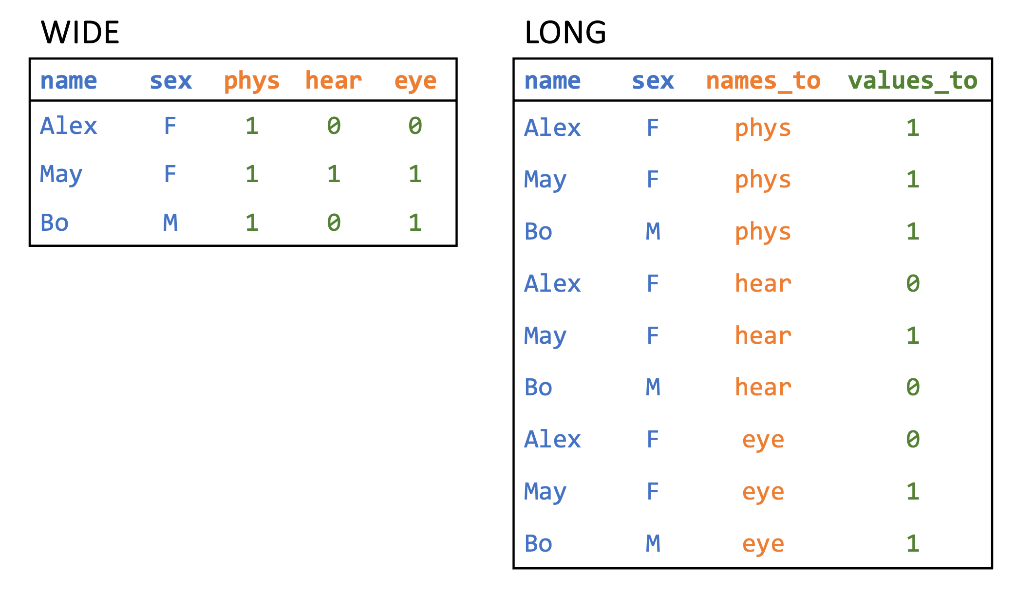
To reshape our data, we use the pivot_longer() function to change the data from what is called wide form to what is called long form. This kind of pivot involves taking a subset of columns that we want to gather into a single column while increasing the number of rows in the dataset. Before pivoting, we have to think about which columns we are transforming. The image in Figure 7.1 shows a picture of some data on whether students have completed a physical, hearing, or eye exam. The data is presented in wide form on the left and long form on the right. To transform wide data to long data, we have identified a subset of columns cols that we want to transform (these cols are phys, hear, and eye in the left table). The long form contains a new column names_to that contains the exam type, and values_to that contains a binary variable indicating whether or not each exam was completed.
In our case, we want to take the lockdown start and end columns and create two new columns: one column will indicate whether or not a date represents the start or end of a lockdown, and the other will contain the date itself. These are called the key and value columns, respectively. The key column gets its values from the names of the columns we are transforming (or the keys), whereas the value column gets its values from the entries in those columns (or the values).
The pivot_longer() function takes in a data table, the columns cols that we are pivoting to longer form, the column name names_to that will store the data from the previous column names, and the column name values_to that will store the information from the columns gathered. In our case, we name the first column Lockdown_Event, since it will contain whether each date is the start or end of a lockdown, and we name the second column Date. Take a look at the result.
lockdown_long <- lockdowndates %>%
  pivot_longer(cols = c("Lockdown_Start", "Lockdown_End"),
               names_to = "Lockdown_Event", values_to = "Date") %>%
  mutate(Date = as.Date(Date, formula ="%Y-%M-%D"),
         Lockdown_Event = ifelse(Lockdown_Event=="Lockdown_Start",
                                 "Start", "End")) %>%
  na.omit()
head(lockdown_long)
#> # A tibble: 6 × 3
#>   State   Lockdown_Event Date
#>   <chr>   <chr>          <date>
#> 1 Alabama Start          2020-04-04
#> 2 Alabama End            2020-04-30
#> 3 Alaska  Start          2020-03-28
#> 4 Alaska  End            2020-04-24
#> 5 Arizona Start          2020-03-31
#> 6 Arizona End            2020-05-16
In R, we can also transform our data in the opposite direction (from long form to wide form instead of from wide form to long form) using the function pivot_wider(). This function again first takes in a data table, but now we specify the arguments names_from and values_from. The former indicates the column that R should get the new column names from, and the latter indicates where the row values should be taken from. For example, in order to pivot our lockdown data back to wide form in the following code, we specify that names_from is the lockdown event and values_from is the date itself. Now we are back to the same form as before!
lockdown_wide <- pivot_wider(lockdown_long,
                             names_from = Lockdown_Event,
                             values_from = Date)
head(lockdown_wide)
#> # A tibble: 6 × 3
#>   State       Start      End
#>   <chr>       <date>     <date>
#> 1 Alabama     2020-04-04 2020-04-30
#> 2 Alaska      2020-03-28 2020-04-24
#> 3 Arizona     2020-03-31 2020-05-16
#> 4 California  2020-03-19 2021-01-25
#> 5 Colorado    2020-03-26 2020-04-27
#> 6 Connecticut 2020-03-23 2020-05-20
Here’s another example: suppose that I want to create a data frame where the columns correspond to the number of cases for each state in New England, and the rows correspond to the numbered months. First, I need to filter my data to New England and then summarize my data to find the number of cases per month. I use the month() function to be able to group by month and state. Additionally, you can see that I add an ungroup() at the end. When we summarize on data grouped by more than one variable, the summarized output is still grouped. In this case, the warning message states that the data is still grouped by state.
ne_cases <- covidcases %>%
  filter(state %in% c("Maine", "Vermont", "New Hampshire",
                      "Connecticut", "Rhode Island",
                      "Massachusetts")) %>%
  mutate(month = month(date)) %>%
  group_by(state, month) %>%
  summarize(total_cases = sum(weekly_cases)) %>%
  ungroup()
head(ne_cases)
#> # A tibble: 6 × 3
#>   state       month total_cases
#>   <chr>       <dbl>       <int>
#> 1 Connecticut     3        7489
#> 2 Connecticut     4       22764
#> 3 Connecticut     5       13640
#> 4 Connecticut     6        2913
#> 5 Connecticut     7        3062
#> 6 Connecticut     8        3031
Now, I need to convert this data to wide format with a column for each state, so my names_from argument is state. Further, I want each row to have the case values for each state, so my values_from argument is total_cases. The format of this data may not be tidy, but it allows me to quickly compare cases across states.
pivot_wider(ne_cases, names_from = state, values_from = total_cases)
#> # A tibble: 7 × 7
#>   month Connecticut Maine Massachusetts `New Hampshire` `Rhode Island`
#>   <dbl>       <int> <int>         <int>           <int>          <int>
#> 1     3        7489   510         14971             744           1006
#> 2     4       22764   716         54704            1875           7513
#> 3     5       13640  1378         33913            2503           5558
#> 4     6        2913   831          6454             807           1426
#> 5     7        3062   540          8841             758           1741
#> # ℹ 2 more rows
#> # ℹ 1 more variable: Vermont <int>
7.2.1 Practice Question
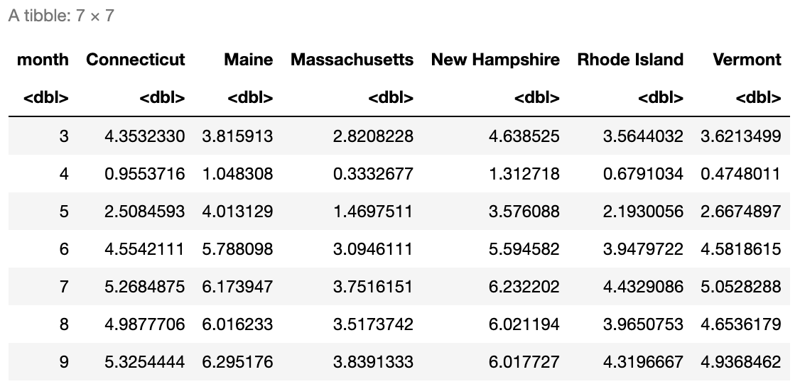
Create a similar data frame as we did in the previous example but this time using the mobility dataset. In other words, create a data frame where the columns correspond to the average mobility for each state in New England, and the rows correspond to the numbered months. You should get a result that looks like in Figure 7.2.
# Insert your solution here:The pivots seen so far were relatively simple in that there was only one set of values we were pivoting on (e.g., the lockdown date, COVID-19 cases). The tidyr package provides examples of more complex pivots that you might want to apply to your data (Wickham, Vaughan, and Girlich 2023).
7.2.2 Pivot Video
In this video, we demonstrate a pivot longer when there is information in the column names, a pivot wider with multiple value columns, and a pivot longer with many variables in the columns.
7.3 Merging Data with Joins
In the last section, we saw how to manipulate our current data into new formats. Now, we see how we can combine multiple data sources. Merging two data frames is called joining, and the functions we use to perform this joining depends on how we want to match values between the data frames. For example, we can join information about age and statin use from table1 and table2 matching by name.
table1 <- data.frame(age = c(14, 26, 32),
                     name = c("Alice", "Bob", "Alice"))
table2 <- data.frame(name = c("Carol", "Bob"),
                     statins = c(TRUE, FALSE))
full_join(table1, table2, by = "name")
#>   age  name statins
#> 1  14 Alice      NA
#> 2  26   Bob   FALSE
#> 3  32 Alice      NA
#> 4  NA Carol    TRUE
The following list gives an overview of the different possible joins. For each join type, we specify two tables, table1 and table2, and the by argument, which specifies the columns used to match rows between tables.
Types of Joins:
left_join(table1, table2, by): Joins each row of table1 with all matches in table2.
right_join(table1, table2, by): Joins each row of table2 with all matches in table1 (the opposite of a left join)
inner_join(table1, table2, by): Looks for all matches between rows in table1 and table2. Rows that do not find a match are dropped.
full_join(table1, table2, by): Keeps all rows from both tables and joins those that match. Rows that do not find a match have NA values filled in.
semi_join(table1, table2, by): Keeps all rows in table1 that have a match in table2 but does not join to any information from table2.
anti_join(table1, table2, by): Keeps all rows in table1 that do not have a match in table2 but does not join to any information from table2. The opposite of a semi-join.
7.3.1 Types of Joins Video
We first demonstrate a left-join using the left_join() function. This function takes in two data tables (table1 and table2) and the columns to match rows by. In a left-join, for every row of table1, we look for all matching rows in table2 and add any columns not used to do the matching. Thus, every row in table1 corresponds to at least one entry in the resulting table but possibly more if there are multiple matches. In the subsequent code chunk, we use a left-join to add the lockdown information to our covidcases data. In this case, the first table is covidcases and we match by state. Since the state column has a slightly different name in the two data frames (“state” in covidcases and “State” in lockdowndates), we specify that state is equivalent to State in the by argument.
covidcases_full <- left_join(covidcases, lockdowndates,
                             by = c("state" = "State"))
head(covidcases_full)
#> # A tibble: 6 × 8
#>   state         county   week weekly_cases weekly_deaths date
#>   <chr>         <chr>   <dbl>        <int>         <int> <date>
#> 1 California    Marin       9            1             0 2020-02-23
#> 2 California    Orange      9            3             0 2020-02-23
#> 3 Florida       Manatee     9            1             0 2020-02-23
#> 4 California    Napa        9            1             0 2020-02-23
#> 5 New Hampshire Grafton     9            2             0 2020-02-23
#> 6 Washington    Spokane     9            4             0 2020-02-23
#> # ℹ 2 more variables: Lockdown_Start <date>, Lockdown_End <date>
These two new columns allow us to determine whether the start of each recorded week was during a lockdown. We use the between() function to create a new column lockdown before dropping the two date columns. We can check that this column worked as expected by choosing a single county to look at.
covidcases_full <- covidcases_full %>%
  mutate(lockdown = between(date, Lockdown_Start, Lockdown_End)) %>%
  select(-c(Lockdown_Start, Lockdown_End))
covidcases_full %>%
  filter(state == "Alabama", county == "Jefferson",
         date <= as.Date("2020-05-10"))
#> # A tibble: 10 × 7
#>   state   county     week weekly_cases weekly_deaths date       lockdown
#>   <chr>   <chr>     <dbl>        <int>         <int> <date>     <lgl>
#> 1 Alabama Jefferson    11           21             0 2020-03-08 FALSE
#> 2 Alabama Jefferson    12           70             0 2020-03-15 FALSE
#> 3 Alabama Jefferson    13          191             0 2020-03-22 FALSE
#> 4 Alabama Jefferson    14          179            12 2020-03-29 FALSE
#> 5 Alabama Jefferson    15          159             4 2020-04-05 TRUE
#> # ℹ 5 more rows
We now want to add in the mobility data. In the previous join, we wanted to keep any observation in covidcases regardless if it was in the lockdowndates data frame. Therefore, we used a left-join. In this case, we only want to keep observations that have mobility data for that state on each date. This indicates that we want to use an inner-join. The function inner_join() takes in two data tables (table1 and table2) and the columns to match rows by. The function only keeps rows in table1 that match to a row in table2. Again, those columns in table2 not used to match with table1 are added to the resulting outcome. In this case, we match by both state and date.
covidcases_full <- inner_join(covidcases_full, mobility,
                              by = c("state", "date")) %>%
  select(-c(samples, m50_index))
head(covidcases_full)
#> # A tibble: 6 × 8
#>   state      county  week weekly_cases weekly_deaths date       lockdown
#>   <chr>      <chr>  <dbl>        <int>         <int> <date>     <lgl>
#> 1 Florida    Okalo…    10            1             0 2020-03-01 FALSE
#> 2 Georgia    Charl…    10            1             0 2020-03-01 FALSE
#> 3 Massachus… Essex     10            1             0 2020-03-01 FALSE
#> 4 New York   Rockl…    10            6             0 2020-03-01 FALSE
#> 5 Indiana    Hendr…    10            2             0 2020-03-01 FALSE
#> 6 California Marin     10            1             0 2020-03-01 FALSE
#> # ℹ 1 more variable: m50 <dbl>
7.3.2 Practice Question
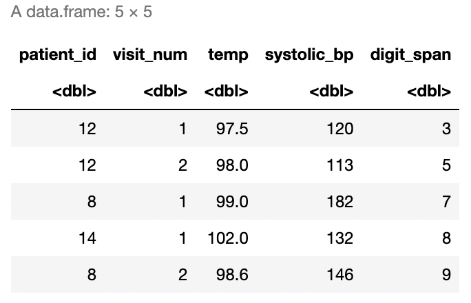
Look at the two data frames, df_A and df_B, defined in the following code. What kind of join would produce the data frame in Figure 7.3? Perform this join yourself.
df_A <- data.frame(patient_id = c(12, 9, 12, 8, 14, 8),
                  visit_num = c(1, 1, 2, 1, 1, 2),
                  temp = c(97.5, 96, 98, 99, 102, 98.6),
                  systolic_bp = c(120, 138, 113, 182, 132, 146))
df_A
#>   patient_id visit_num  temp systolic_bp
#> 1         12         1  97.5         120
#> 2          9         1  96.0         138
#> 3         12         2  98.0         113
#> 4          8         1  99.0         182
#> 5         14         1 102.0         132
#> 6          8         2  98.6         146
df_B <- data.frame(patient_id = c(12, 12, 12, 8, 8, 8, 14, 14),
                   visit_num = c(1, 2, 3, 1, 2, 3, 1, 2),
                   digit_span = c(3, 5, 7, 7, 9, 5, 8, 7))
df_B
#>   patient_id visit_num digit_span
#> 1         12         1          3
#> 2         12         2          5
#> 3         12         3          7
#> 4          8         1          7
#> 5          8         2          9
#> 6          8         3          5
#> 7         14         1          8
#> 8         14         2          7
# Insert your solution here:7.4 Exercises
Take a look at the provided code. What is wrong with it? Hint: think about what causes the warning message.
visit_info <- data.frame(
  name.f = c("Phillip", "Phillip", "Phillip", "Jessica",
             "Jessica"),
  name.l = c("Johnson", "Johnson", "Richards", "Smith",
             "Abrams"),
  measure = c("height", "age", "age", "age", "height"),
  measurement = c(45, 186, 50, 37, 156)
)

contact_info <- data.frame(
first_name = c("Phillip", "Phillip", "Jessica", "Margaret"),
last_name = c("Richards", "Johnson", "Smith", "Reynolds"),
email = c("pr@aol.com", "phillipj@gmail.com",
          "jesssmith@brown.edu", "marg@hotmail.com")
)

left_join(visit_info, contact_info,
          by = c("name.f" = "first_name"))
#> Warning in left_join(visit_info, contact_info, by = c(name.f = "first_name")): Detected an unexpected many-to-many relationship between `x` and `y`.
#> ℹ Row 1 of `x` matches multiple rows in `y`.
#> ℹ Row 1 of `y` matches multiple rows in `x`.
#> ℹ If a many-to-many relationship is expected, set `relationship =
#>   "many-to-many"` to silence this warning.
#>    name.f   name.l measure measurement last_name               email
#> 1 Phillip  Johnson  height          45  Richards          pr@aol.com
#> 2 Phillip  Johnson  height          45   Johnson  phillipj@gmail.com
#> 3 Phillip  Johnson     age         186  Richards          pr@aol.com
#> 4 Phillip  Johnson     age         186   Johnson  phillipj@gmail.com
#> 5 Phillip Richards     age          50  Richards          pr@aol.com
#> 6 Phillip Richards     age          50   Johnson  phillipj@gmail.com
#> 7 Jessica    Smith     age          37     Smith jesssmith@brown.edu
#> 8 Jessica   Abrams  height         156     Smith jesssmith@brown.edu
First, use the
covidcasesdata to create a new data frame calledsub_casescontaining the total number of cases by month for the states of California, Michigan, Connecticut, Rhode Island, Ohio, New York, and Massachusetts. Then, manipulate themobilitydata to calculate the averagem50mobility measure for each month. Finally, merge these two datasets using an appropriate joining function.Convert the
sub_casesdata frame from the previous exercise to wide format so that each row displays the cases in each state for a single month. Then, add on the average m50 overall for each month as an additional column using a join function.