1 Getting Started with R

This chapter introduces you to R as a programming language and show you how we can use this language in two different ways: directly through the R console and using the RStudio development environment. To start, you need to download R and RStudio.

1.1 Why R?

What are some of the benefits of using R?

R is built for statisticians and data analysts.
R is open source.
R has most of the latest statistical methods available.
R is flexible.

Since R is built for statisticians, it is built with data in mind. This comes in handy when we want to streamline how we process and analyze data. It also means that many statisticians working on new methods are publishing user-created packages in R, so R users have access to most methods of interest. R is also an interpreted language, which means that we do not have to compile our code into machine language first: this allows for simpler syntax and more flexibility when writing our code, which also makes it a great first programming language to learn.

Python is another interpreted language often used for data analysis. Both languages feature simple and flexible syntax, but while python is more broadly developed for usage outside of data science and statistical analyses, R is a great programming language for those in health data science. I use both languages and find switching between them to be straightforward, but I do prefer R for anything related to data or statistical analysis.

1.1.1 Installation of R and RStudio

To run R on your computer, you need to download and install R. This allows you to open the R application and run R code interactively. However, to get the most out of programming with R, you should install RStudio, which is an integrated development environment (IDE) for R. RStudio offers a nice environment for writing, editing, running, and debugging R code.

Each chapter in this book is written as a Quarto document and can also be downloaded as a Jupyter notebook. You can open Quarto files in RStudio to run the code as you read and complete the practice questions and exercises.

1.2 The R Console

The R console provides our first intro to code in R. Figure 1.1 shows the console appearance when opened. You should see a blinking cursor - this where we can write our first line of code!

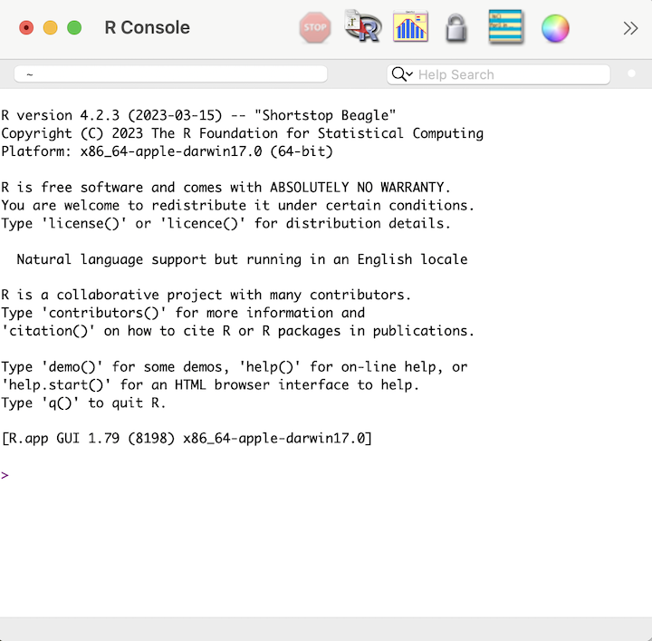
To start, type 2+3 and press ENTER. You should see that 5 is printed below that code and that your cursor is moved to the next line.

1.2.1 Basic Computations and Objects

In the previous example, we coded a simple addition. Try out some other basic calculations using the following operators :

Addition: 5+6
Subtraction: 7-2
Multiplication: 2*3
Division: 6/3
Exponentiation: 4^2
Modulo: 100 %% 4

For example, use the modulo operator to find what 100 mod 4 is. It should return 0 since 100 is divisible by 4.

If we want to save the result of any computation, we need to create an object to store our value of interest. An object is simply a named data structure that allows us to reference that data structure. Objects are also commonly called variables. In the following code, we create an object x which stores the value 5 using the assignment operator <-. The assignment operator assigns whatever is on the right hand side of the operator to the name on the left hand side. We can now reference x by calling its name. Additionally, we can update its value by adding 1. In the second line of code, the computer first finds the value of the right hand side by finding the current value of x before adding 1 and assigning it back to x.

x <- 2+3
x <- x+1
x
#> [1] 6

We can create and store multiple objects by using different names. The following code creates a new object y that is one more than the value of x. We can see that the value of x is still 5 after running this code.

x <- 2+3
y <- x
y <- y + 1
x
#> [1] 5

1.2.2 Naming Conventions

As we start creating objects, we want to make sure we use good object names. Here are a few tips for naming objects effectively:

Stick to a single format. We use snake_case, which uses underscores between words (e.g. my_var, class_year).
Make your names useful. Try to avoid using names that are too long
(e.g. which_day_of_the_week) or do not contain enough information (e.g., x1, x2, x3).
Replace unexplained numeric values with named objects. For example, if you need to do some calculations using 100 as the number of participants, create an object n_part with value 100 rather than repeatedly using the number. This makes the code easy to update and helps the user avoid possible errors.

1.3 RStudio and Quarto

If we made a mistake in the code we type in the console, we would have to re-enter everything from the beginning. However, when we write code, we often want to be able to run it multiple times and develop it in stages. R scripts and R markdown files allow us to save all of our R code in files that we can update and re-run, which allows us to create reproducible and easy-to-share analyses. We now move to RStudio as our development environment to demonstrate creating an R script. When you open RStudio, there are multiple windows. Start by opening a new R file by going to File -> New File -> R Script. You should now see several windows as outlined in Figure 1.2.

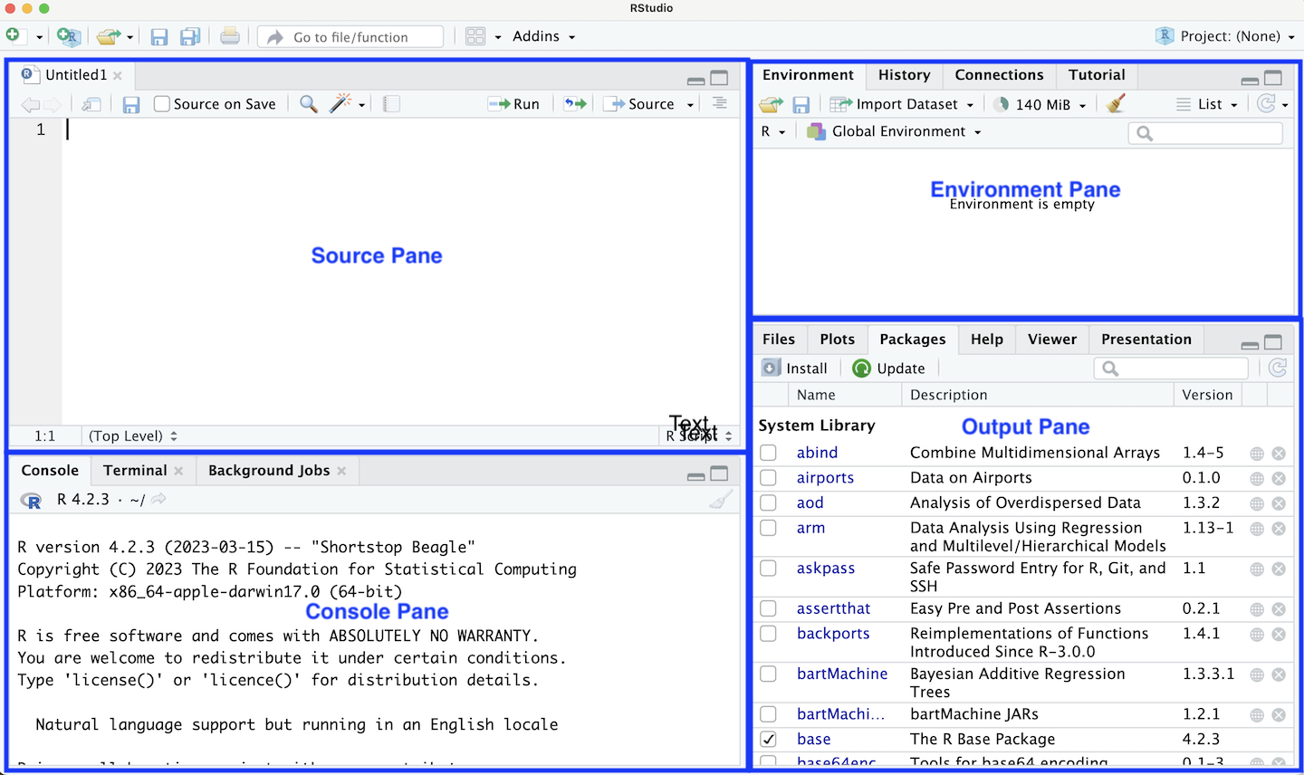
1.3.1 Panes

There are four panes shown by default:

Source Pane - used for editing code files such as R scripts or Quarto documents.
Console Pane - used to show the live R session.
Environment Pane - containing the Environment and History tabs, used to keep track of the current state.
Output Pane - containing the Plots and Packages tabs.

The source pane is the code editor window in the top left. This shows your currently blank R script. Add the following code to your .R file and save the file as “test.R”. Note that here we used snake_case to name our objects!

# Calculate primary care physician to specialist ratio
pcp_phys <- c(6300, 1080, 9297, 16433)
spec_phys <- c(6750, 837, 10517, 22984)
pcp_spec_ratio <- 1000 * pcp_phys / spec_phys

The first line starts with # and does not contain any code. This is a comment line, which allows us to add context, intent, or extra information to help the reader understand our code. A good rule of thumb is that we want to write enough comments so that we could open our code in six months and be able to understand what we were doing. As we develop longer chunks of code, this will become more important.

Unlike when we type code into the console, we can write multiple lines of code in our R script without running them. In order to run the code in the script, we need to tell RStudio we are ready to run it. To run a single line of code, we can either hit Ctrl+Enter when on that line or we can hit the Run button 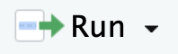button at the top right of the source pane. This copies the code to the R Console. Try this out to run the first line of code that defines pcp_phys. You can see that the line of code has been run in the console pane. Now check your environment pane. You should see that you have a new object representing the one we just created. This pane keeps track of all current objects. Run the second line of code and see how the environment updates. If you look at the History tab within this pane, you see the history of R commands run.

If we want to run all lines of code in our script, we can use the Source button 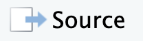. Before we do this, we will clear our environment. You can do this by clicking the broom in the environment pane, which deletes all objects in the environment. Alternatively, you can go to Session -> Restart R in the main menu, which restarts your whole R session. After clearing your environment, click the source button. You will see that in the R console it shows that it sourced this file. This means that it runs through all lines of code in this file. You can see that our objects have been added back into our environment.

source("test.R")

Now suppose we want to update our script by adding a plot. Copy the code in subsequent code chunk, save your updated file, and then source your file. You will see that the generated plot will appear in your output pane.

plot(spec_phys, pcp_phys)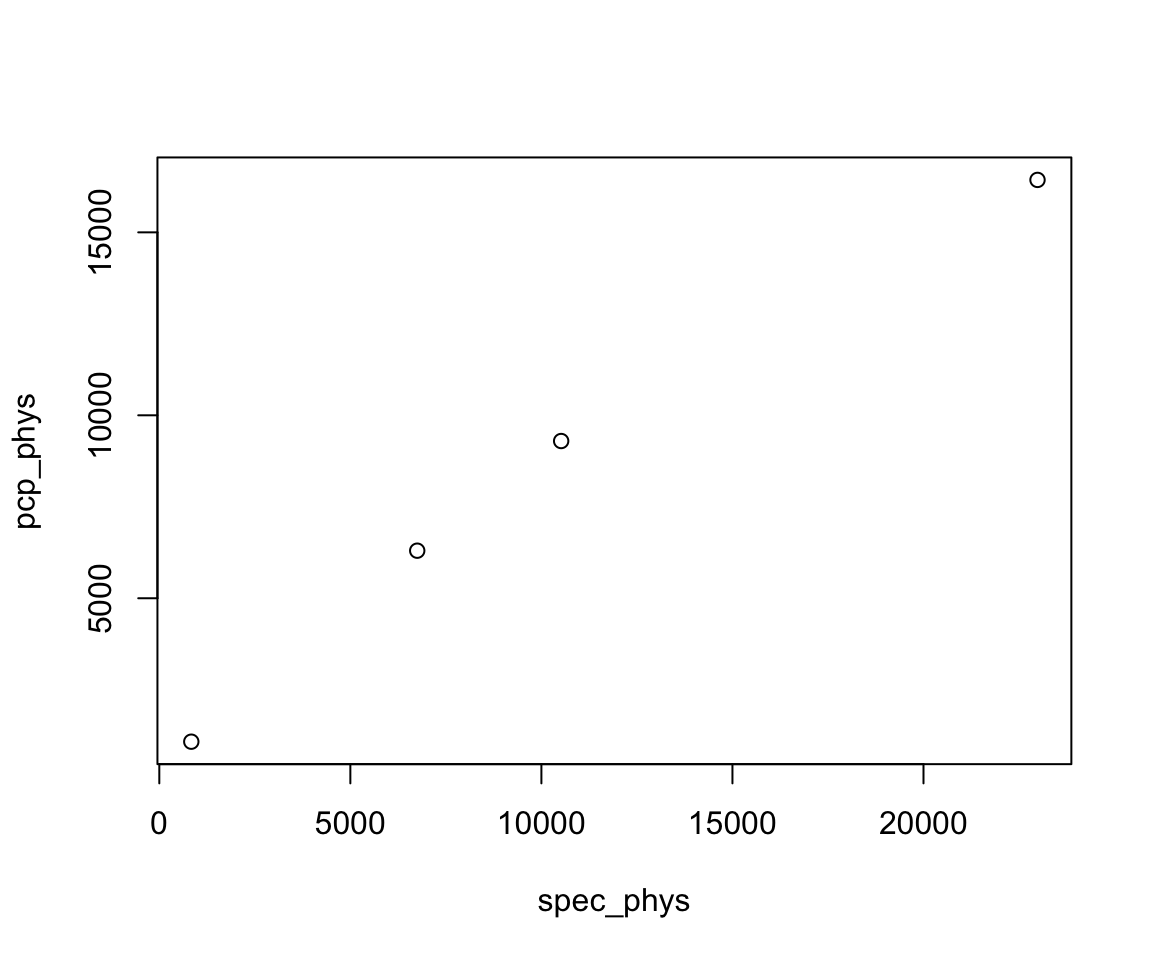

Unlike R scripts which only contain R code, Quarto documents allow us to intersperse text and code. This breaks our code into chunks surrounded by text written in markdown. Every chapter in this book is available as a Quarto document. Try opening the Quarto file for Chapter 2 of this book. You will see the first code chunk as in Figure 1.3. In order to run the code in a code chunk, we can again use Ctrl+Enter to run a single line or selected lines. Additionally, we can use the Play button . This runs all the code within the chunk. We recommend using the available Quarto documents to follow along with the text. Writing your own Quarto documents is covered in Chapter 22.

1.3.2 Video Tour of RStudio and R Markdown

This video reviews the layout of RStudio as well as how to run and write R scripts and Quarto files.

1.3.3 Calling Functions

When we use R, we have access to all the functions available in base R. A function takes in one or more inputs and returns a single output object. Let’s first use the simple function exp(). This exponential function takes in one (or more) numeric values and exponentiates them. The following code computes \(e^3\).

exp(3)
#> [1] 20.1

Some other simple functions are shown that all convert a numeric input to an integer value. The ceiling() and floor() functions returns the ceiling and floor of your input, and the round() function round your input to the closest integer. Note that the round() function rounds a number ending in 0.5 to the closest even integer.

ceiling(3.7)
#> [1] 4

floor(3.7)
#> [1] 3

round(2.5)
#> [1] 2
round(3.5)
#> [1] 4

If we want to learn about a function, we can use the help operator ? by typing it in front of the function you are interested in: this brings up the documentation for that particular function. This documentation often tells you the usage of the function, the arguments (the object inputs), the value (information about the returned object), and gives some examples of how to use the function. For example, if we want to understand the difference between floor() and ceiling(), we can call ?floor and ?ceiling. This should bring up the documentation in your help window. We can then read that the floor function rounds a numeric input down to the nearest integer whereas the ceiling function rounds a numeric input up to the nearest integer.

1.3.4 Working Directories and Paths

Let’s try using another example function: read.csv(). This function reads in a comma-delimited file and returns the information as a data frame (try typing ?read.csv in the console to read more about this function). We learn more about data frames in Chapter 2. The first argument to this function is a file, which can be expressed as either a file name or a path to a file. First, download the file fake_names.csv from this book’s github repository. By default, R looks for the file in your current working directory To find the working directory, you can run getwd(). You can see in the following output that my current working directory is where the book content is on my computer.

getwd()
#> [1] "/Users/Alice/Dropbox/health-data-science-using-r/book"

You can either move the .csv file to your current working directory and load it in, or you can specify the path to the .csv file. Another option is to update your working directory by using the setwd() function.

setwd('/Users/Alice/Dropbox/health-data-science-using-r/book/data')

If you receive an error that a file cannot be found, you most likely have the wrong path to the file or the wrong file name. In the following code, I chose to specify the path to the downloaded .csv file, saved this file to an object called df, and then printed that df object.

# update this with the path to your file
df <- read.csv("data/fake_names.csv") 
df
#>                  Name Age     DOB            City State
#> 1           Ken Irwin  37 6/28/85      Providence    RI
#> 2 Delores Whittington  56 4/28/67      Smithfield    RI
#> 3       Daniel Hughes  41 5/22/82      Providence    RI
#> 4         Carlos Fain  83  2/2/40          Warren    RI
#> 5        James Alford  67 2/23/56 East Providence    RI
#> 6        Ruth Alvarez  34 9/22/88      Providence    RI

We can see that df contains the information from the .csv file and that R has printed the first few observations of the data.

1.3.5 Installing and Loading Packages

When working with data frames, we often use the tidyverse package (Wickham 2023), which is actually a collection of R packages for data science applications. An R package is a collection of functions and/or sample data that allow us to expand on the functionality of R beyond the base functions. You can check whether you have the tidyverse package installed by going to the package tab in the Output Pane in RStudio or by running the following command, which displays all your installed packages.

installed.packages()

If you don’t already have a package installed, you can install it using the install.packages() function. Note that you have to include single or double quotes around the package name when using this function. You only have to install a package one time.

install.packages('tidyverse')

The function read_csv() is another function to read in comma-delimited files that is part of the readr package in the tidyverse (Wickham, Hester, and Bryan 2023). However, if we tried to use this function to load in our data, we would get an error that the function cannot be found. That is because we haven’t loaded in this package. To do so, we use the library() function. Unlike the install.packages() function, we do not have to use quotes around the package name when calling this library() function. When we load in a package, we see some messages. For example, in the following output we see that this package contains the functions filter() and lag() that are also functions in base R. In future chapters, we suppress these messages to make the chapter presentation nicer. After loading the tidyverse package, we can now use the read_csv() function.

library(tidyverse)

df <- read_csv("data/fake_names.csv", show_col_types=FALSE)
df
#> # A tibble: 6 × 5
#>   Name                  Age DOB     City            State
#>   <chr>               <dbl> <chr>   <chr>           <chr>
#> 1 Ken Irwin              37 6/28/85 Providence      RI   
#> 2 Delores Whittington    56 4/28/67 Smithfield      RI   
#> 3 Daniel Hughes          41 5/22/82 Providence      RI   
#> 4 Carlos Fain            83 2/2/40  Warren          RI   
#> 5 James Alford           67 2/23/56 East Providence RI   
#> 6 Ruth Alvarez           34 9/22/88 Providence      RI

Alternatively, we could have told R where to locate the function by adding readr:: before the function. This tells it to find read_csv() function in the readr package. This can be helpful even if we have already loaded in the package, since sometimes multiple packages have functions with the same name.

df <- readr::read_csv("data/fake_names.csv", show_col_types = FALSE)

1.4 RStudio Projects and RStudio Global Options

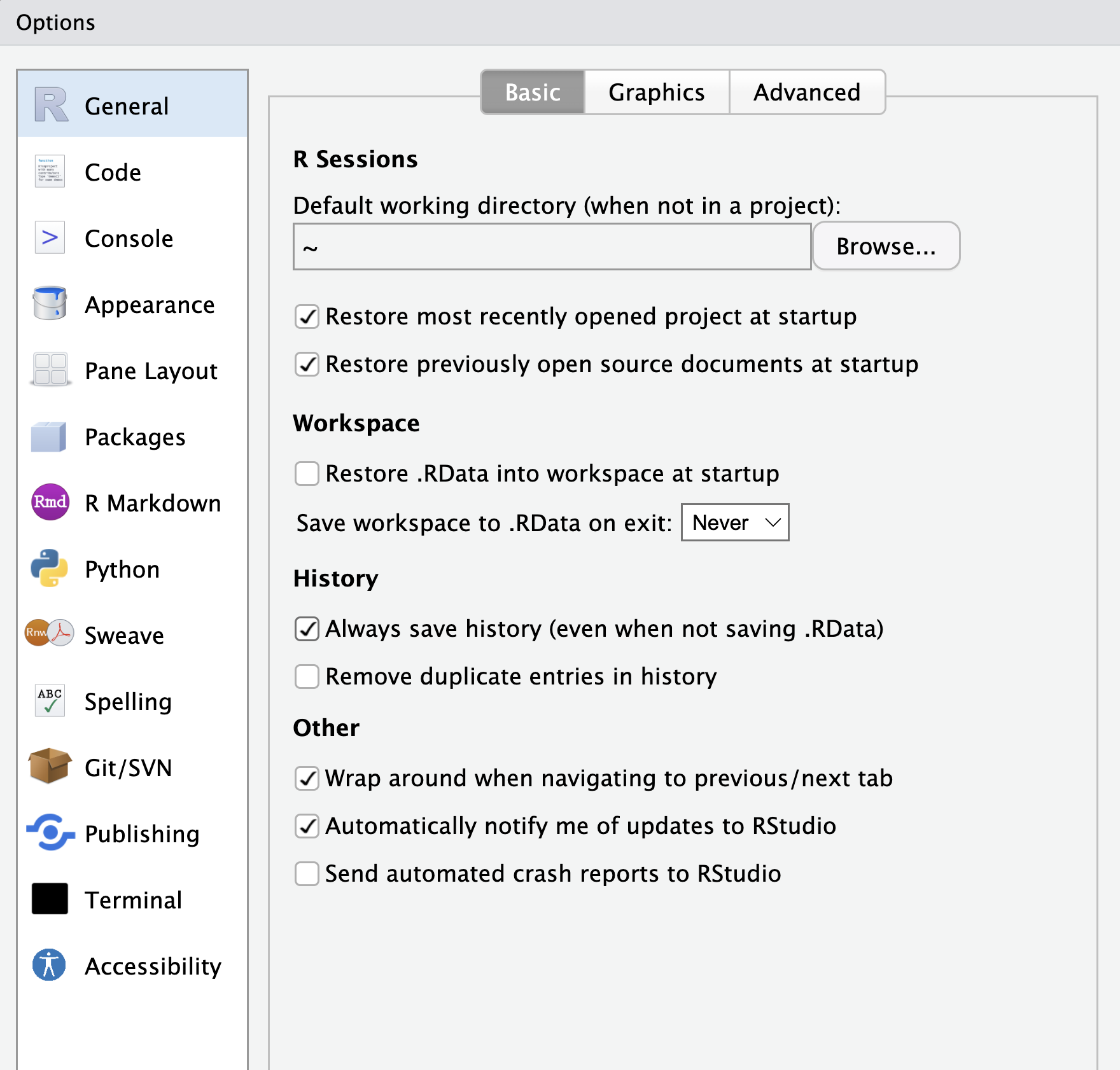
You have now had a basic tour of RStudio. Once you close RStudio, you have the option of whether to store your current R environment. We highly recommend that you update your RStudio options to not save your workspace on exiting or load it on starting. This ensures that you have a fresh environment every time you open RStudio and helps you to create fully reproducible code and avoid possible errors or confusion.

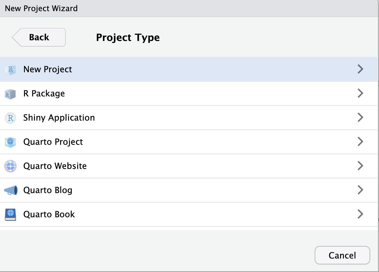
Now when you re-open RStudio, it opens the files you had open previously and has your history of commands. This may become confusing when you are working on different files. RStudio projects allow us to create a folder that are associated with a single project. This means that when we open our project it sets the appropriate work directory for us and only open files related to that project. In order to create a new R project, such as one associated with this book, you can go to File -> New Project. You can then choose whether to create a new directory or existing directory before selecting to create an empty project as in Figure 1.5. Within this directory you should see a .RProj file that allows you to re-open your project.

Figure 1.5: Creating a New RStudio Project.

1.5 Tips and Reminders

We end this chapter with some final tips and reminders.

Keyboard Shortcuts: RStudio has several useful keyboard shortcuts that make your programming experience more streamlined. It is worth getting familiar with some of the most common keyboard shortcuts using this book’s cheatsheet.
Asking for help: Within R, you can use the ? operator or the help() function to pull up documentation on a given function. This documentation is also available online.
Finding all objects: You can use the environment pane or ls() function to find all current objects. If you have an error that an object you are calling does not exist, take a look to find where you defined it.
Checking packages: If you get an error that a function does not exist, check to make sure you have loaded that package using the library() function. The list of packages used in this book is given on the github repository homepage.